(Written jointly with Jens von Bergmann and cross-posted at MountainMath)

TL;DR

We develop and elaborate a Montréal Method for estimating housing shortfalls related to constraints upon current residents who might wish to form independent households but are forced to share by local housing markets. Applying simple versions of the Montréal Method to Metro Areas across Canada suggests that Toronto has the biggest shortfall, which we estimate at 250,000 to 400,000 dwellings, depending upon assumptions. For Vancouver, the estimated shortfall range is narrower, from roughly 75,000 to 100,000 dwellings. But models suggest housing shortfalls remain widespread, and there is much room for further elaboration. Note: shortfalls estimated in this post only account for those due to suppressed household formation among residents and do not account for e.g. migration pressures, which means that overall housing shortfalls are likely much larger.

Intro

In a previous post we tried to explain what goes wrong with population and dwelling growth projections in planning. In this post we will examine household maintainer rates more closely, one of the two key places where implicit model assumptions perpetuate and amplify housing scarcity. We’ll also lay out adjustments to consider that we’ll call “The Montréal Method” for estimating housing needs based on suppressed household formation.

Household maintainer rates, sometimes called headship rates, are the share of the population 15+, or within a specific age group, who are coded as “primary household maintainer” in the census. The concept draws upon an older & occasionally patriarchal notion of household head, where the census was interested in identifying who was “in charge” of the household, and updates it by merely identifying the first person listed who pays the bills. Often, of course, as with most couples, there are two or more people paying the bills. But only one gets identified as the “primary” household maintainer in order to help identify a single link between households and the people they contain. Correspondingly, household maintainer rates serve as a sort of missing link in how we fit populations into dwellings. This missing link also contains information about household size. And as we noted previously with respect to Metro population projections, assumptions about household maintainer rates have a significant impact on housing needs and demand estimates.

Often housing needs and demand projections assume household maintainer rates will follow past trends, but as explained in our previous post this assumption tends to enshrine and worsen past housing shortages. If in the past housing was scarce, and household maintainer rates have been suppressed by, e.g. delaying independent household formation of young adults, simply projecting past trends forward would bake these past shortages into plans for the future. In other words, normal planning processes, as with Metro Vancouver’s growth projections, can serve to systematically enshrine housing shortages.

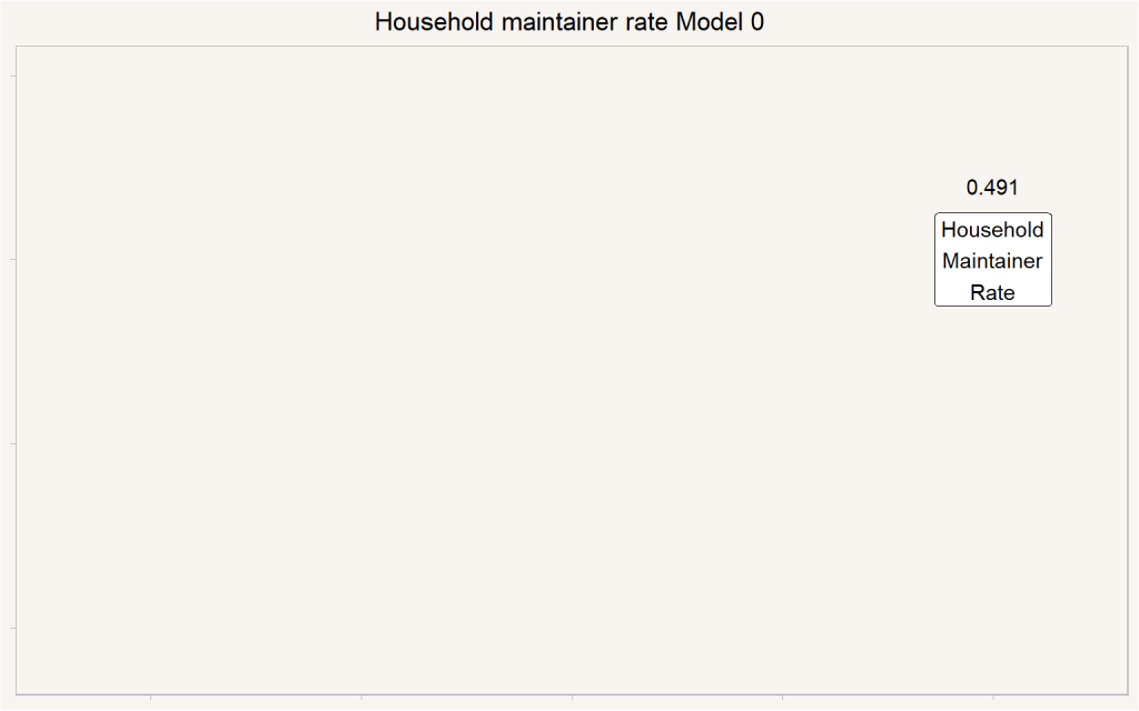
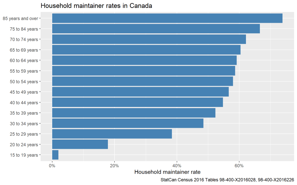
As a start, let’s estimate recent household maintainer rates in Canada for the population 15 years or older. Our figure comes out to 49%. That’s the factor we need to multiply the population 15 years or older by to get to our estimated number of private households. It tells us what to put into the ‘Household Maintainer Rate’ box on the diagram in the previous post. In other words, in Canada the average household size is just over 2, if we don’t count children under the age of 15.

We can think of this number as constituting model zero for how to integrate household maintainer rates into linking population to housing.

Household maintainer rates vary across CMAs

Model zero provides a starting number to link population to dwellings. But household maintainer rates aren’t constant across the country; some CMAs have higher household maintainer rates than others. In fact, this is at the core of what we are interested in in this post. How should we understand this variation?

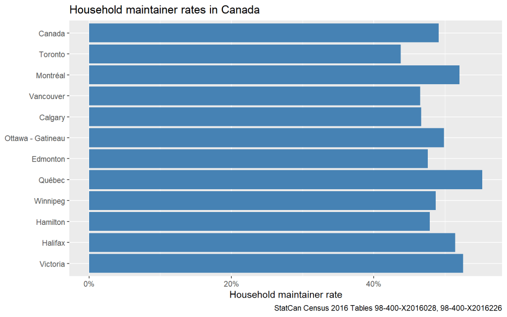
The central question is what causes discrepancies between e.g. Toronto with a household maintainer rate of 45% and Montréal with a rate of 51%? One candidate that immediately comes to mind is the availability of housing. We can encode that in an extension of our Model 0 by explicitly acknowledging that CMA can impact household maintainer rates.

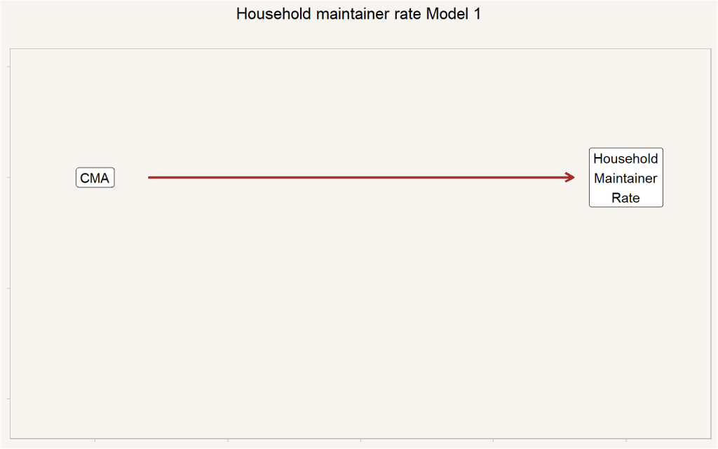
This is still somewhat simplistic, but if we assume that our Model 1 is complete, that CMA variation can be explained by housing constraints, and that there aren’t any other important factors linking CMAs to household maintainer rates, we can ask how much more housing each of these CMAs would need in order to achieve the same household maintainer rates as any other given Metro Area.

Which metro area should we use as our counterfactual of unconstrained household formation? We could use Canada as a whole, of course, but that would just be balancing constrained and unconstrained areas (and there have recently been suggestions that the country as a whole should be understood as in housing deficit). Quebec City is tempting as the metro area with the highest household maintainer rate. But it’s also somewhat small and might be distinct for other reasons. By contrast, Montreal looks like a nice, big, reasonable counterfactual, enabling us to ask how much more housing would other metros need to reach the household maintainer rate of Montreal?

To see if this is reasonable, let’s do a quick preliminary check-in on vacancy rates in the lead-up to our 2016 household maintainer rates as another measure of how they might plausibly have been influenced by housing conditions.

Here we can see patterns that generally support, but might also complicate our understanding of household maintainer rates being linked to housing conditions. Toronto and Vancouver, of course, have notoriously low rental vacancy rates, which match well onto their low household maintainer rates. People can’t readily find apartments to rent, and it’s been that way for awhile. But Victoria’s vacancy rates are also quite low, despite the area having a high household maintainer rate. Québec’s vacancy rates climbed to a high just prior to the 2016 Census that might help explain its high household maintainer rate, but leave concerns about whether it was a temporary effect. Yet Edmonton and Calgary’s rental vacancy rates climbed even more dramatically, while their household maintainer rates aren’t much different from Vancouver’s. It may be the case that fluctuations in vacancy rates take some time to translate into household maintainer rates, but we’re not sure.

This perhaps furthers the case for using Montréal as our counterfactual. Montréal is a big metro area with rental vacancy rates that have remained relatively stable within the 3%-4% range, with high household maintainer rates, if not the highest. So we’re going to go ahead and use Montréal as our baseline to provide estimates for how household formation might be suppressed elsewhere across Canada. And we’re going to call it The Montréal Method.

How much more housing would other metro areas need to reach household maintainer rates matching Montréal’s?

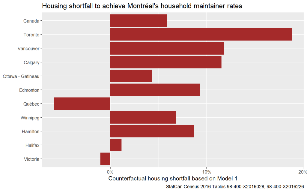
Interesting! But our initial results from The Montréal Method could easily be questioned. Toronto and Vancouver registering with a large housing shortfall seems in principle plausible, but what about Calgary? Does Toronto really need 18% more dwellings to accommodate all those desiring an independent household? And why do Québec City and Victoria appear to have an excess of housing? We might be missing something.

It’s also a good time to remember that the housing shortfall estimated here is only the shortfall due to suppressed household formation, and it disregards housing shortfall due to other factors, for example suppressed in-migration or forced out-migration. Still, it’s a start.

Household maintainer rates vary by age

Time to get a bit more serious. Most household maintainer rate models, including the Metro Vancouver projection models, stratify by age groups. And for good reason! For any given year, age is the strongest predictor for household maintainer rates. The household maintainer rates for 15 year olds are essentially zero. But household maintainer rates generally increase with age and for seniors they rise well over 60%.

Correspondingly, if different CMAs have different age distributions, that might skew our estimates. This tells us we need to refine our Model 1 to account for Age. Here we think of people sorting into CMAs by age, with some CMAs skewing younger and others skewing older. Victoria, for instance, is regularly promoted as “Canada’s Retirement Capital.”

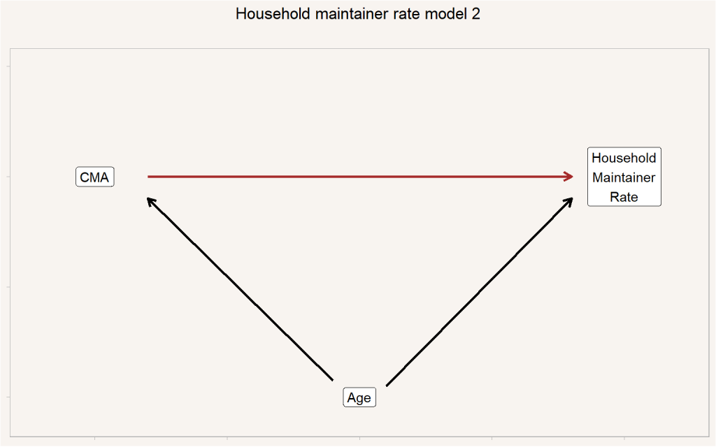
Part of the justification of using household maintainer rates to translate between population and dwellings is the recognition that in most situations all household maintainers in a given household are of similar age, and thus the choice of “primary” household maintainer does not impact these kind of estimates much. Based on this model we can estimate age-adjusted household maintainer rates for each CMA by weighting age specific rates by the overall age distribution in Canada.

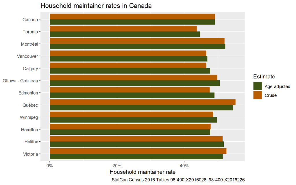
Adjusting by age highlights how some of the difference in household maintainer rates can be accounted for by difference in age distribution across municipalities. In particular, Toronto has a younger than average age distribution whereas Victoria is on average older, so the adjustments go in opposite directions. Nevertheless, the differences across CMA are quite stubborn, only Montréal and Victoria flipped positions in our lineup.

In other words, adjusting for age reduces the variation in household maintainer rates across CMAs a little, by 27% to be precise, but there is still considerable variation left. We can again estimate how many more housing units we would need to achieve the same household maintainer rates as Montréal, after accounting for differences in the age distributions.

Assuming age offers our only important household maintainer determinant and Montréal makes a good counterfactual for where other metro areas could be, this offers us a nice estimate of how much housing we would need to reach Montréal levels of maintainer rates. The Age-Adjusted Montréal Method estimates Vancouver is short well over 10% and Toronto by well over 15%, but shortfalls still appear to be common across most Canadian metro areas, save for Québec.

Age-Specific Metro Household Maintainer Rates across History

Let’s examine our counterfactual a little more carefully by comparing age-specific household maintainer rates directly and taking them backward in time. History gives us another view into the differences in household maintainer rates across CMAs that we have observed above. Have these differences been stable over time, or have they changed significantly? Here we’ll just focus on the historical data we have on age-specific household maintainer rates from 1971-2016 PUMF data for Montréal, Toronto and Vancouver CMAs.

Of note, we have to switch our data source to allow more flexibility. So far we have used data from census cross tabulations, going forward we need to cut data in more custom ways and will rely on PUMF data. In this overview we gloss over a couple of complications, we just use standard weights and don’t show confidence intervals for PUMF estimates, and we ignore that the geographic boundaries of CMAS, in particular Montréal, have changed over time. The broad effects we are trying to highlight here are large enough that they can’t be explained by variability in the PUMF, and we believe that the changing geography won’t have significant effects on the age-specific household maintainer rates in either direction. We talk about the different data sources more in our appendix.

First we compare how age-specific household maintainer rates have changed over time in each of the CMAs.

What does Montréal offer as a counterfactual? Strikingly, age-specific household maintainer rates in Montréal have remained fairly constant over time. The most notable trend is for older age groups, especially age 75+, where we can see a rise in independent living during the 1970s and 1980s, as reflected in rising household maintainer rates.

Comparing Montréal to Toronto and Vancouver, we can see that they had quite similar age-specific household maintainer rates in the 1970s. Then rates in Toronto and Vancouver began to plummet to quite a bit below Montréal’s rates from 2000 onward. These drops are most evident in the age ranges from 25-39, but they also show up in older ranges, with ages 75-79 most notable for Vancouver.

We can slice the data differently and compare the CMAs next to each other over the years.

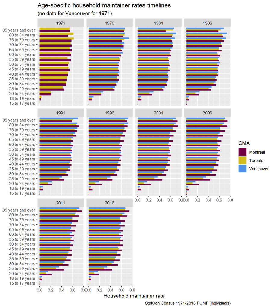
This highlights how similar all three CMAs were in the 1970s, strengthening the case for Montréal as a reasonable counterfactual. Montréal didn’t pull ahead in the 1980s and 1990s so much as Toronto and Vancouver fell behind. The graphic effect is kind of like receding gums gradually leaving Montréal’s teeth exposed.

Let’s leave dentistry behind and return to thinking about housing. Using our Montréal Method can provide estimates of how much housing would be needed to return Toronto and Vancouver to similar household maintainer rates as Montréal, and correspondingly to similar rates reflecting where they were in the 1970s. But is it reasonable to assume that the divergence between these three metro areas is entirely about housing constraints?

Let’s add one more complicating factor: culture.

Cultural Differences?

Perhaps cultural differences emerging in Toronto and Vancouver have altered their trajectories away from their past patterns and away from Montréal’s. These could be associated with the quite different immigration patterns we’ve seen in Toronto and Vancouver. The important idea here is that maybe some of the variation in household maintainer rates has less to do with housing constraints than with different ideas about family and ideal living situations. Maybe some groups of young adults don’t want to live on their own? Maybe some groups of seniors similarly prefer to live with their children?

This leads us to the next refinement of our household maintainer model. There is literature on large cultural differences, and those differences have complex fault lines. For example young adults leave home much later in south and eastern European countries like Italy, Greece, or Spain than in north and western European countries. There are similar arguments to be made about various cultural differences across Asia. For instance, Statistics Canada estimates that South Asian Canadians are over three times as likely to live in complex, multi-family households compared to Canadians as a whole. So we should probably consider ethnic background, but also immigrant generation status. First generation immigrants may have few other options than forming households at high rates, as they often have no parents or support networks to fall back on. Second generation immigrants might stay longer living with their parents, whereas their third or higher generation counterparts may converge toward broader Canadian patterns. We will loosely refer to the intersections of these variables as potentially pointing out differences in Culture.

This tells us that ethnic background, as well as immigrant generation, will likely have an impact on household maintainer rates. We also think of immigrants sorting by cultural background into CMAs, for example based on existing networks.

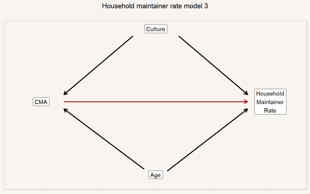
But this is where things get tricky for several reasons. For one, the concepts of ethnic background are somewhat fluid and hard to nail down. A more technical reason is that we are forced to move the analysis to PUMF data, which is roughly a 1:40 subsample of the population, and we are quickly running up against model complexity limits. The PUMF data is simply not thick enough to be able to expect robust estimates of counterfactual model when simultaneously accounting for CMA, Age, and Culture unless we distill Culture down to very broad categories. This is somewhat in keeping with our approach of successively refining our model.

To derive broad categories of Culture we first recode generation status into three groups, First Generation (born outside of Canada), Second Generation (both parents first generation) and all other. Then we manually group the 49 ethnic origin categories that are split out in the PUMF into broader groups. After that we cross the ethnicity categories with the generation status, and collapse some categories further in order to ensure the categories are thick enough to yield somewhat robust estimates. Then we take data from Canada outside of Vancouver and Toronto (where we know housing is constrained) to estimate overall household maintainer rates for these categories and cluster them to arrive at three broad Culture categories (C1, C2, and C3) we will use in our model, the results of which are depicted here.

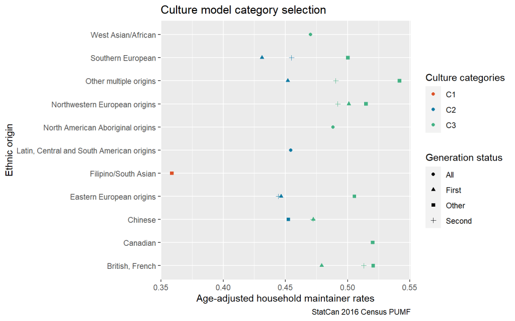
We’re the first to admit that our C1, C2, and C3 “Cultural” groupings linked to different household maintainer patterns are rough. But they allow us to make another pass at understanding differences across metro areas and applying our Montréal Method. With this set up we now have three different models to estimate counter-factual household maintainer rates. The crude estimates, the age-adjusted model and the model adjusting for age and ethnic/immigration background.

We can express this in terms of household maintainer rates as observed using Montréal as counterfactual.

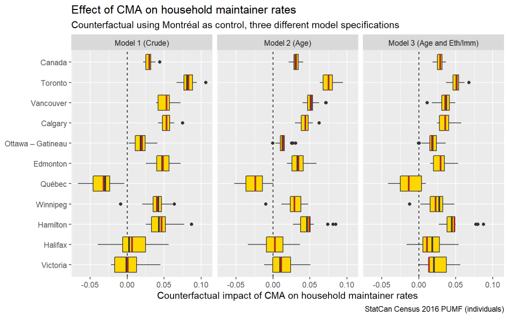
Or, following our Montréal Method, we can express this directly as housing shortfall relative to our counter-factual of Montréal. This corresponds to three different versions of our Montréal Method which we can use to estimate the housing shortfall in other metro areas. Results from the Montréal Method are interpretable as the number of extra dwellings we’d need to enable people to maintain independent households like they do in Montréal. We’ve now established a crude version, and age adjusted version, and a version adjusted for both age and ethnic/immigration background.

This shows how our successively refined models lead to adjustments in the counterfactual effect of CMA on household maintainer rates. We can see how each refinement of the model adjusts the rates of household suppression and associated housing shortfall relative to the counter-factual of Montréal. Adjusting additionally for ethnic background and immigration generation leads to noticeable shifts both up and down. In particular, Toronto’s counter-factual estimates decrease significantly, along with estimates for Vancouver and Calgary. By contrast, Hamilton remains roughly the same.

Overall, in terms of enabling people to form independent households, large swathes of Canada appear to be constrained relative to Montréal. The Québec City CMA alone consistently comes out with a negative housing shortfall, perhaps hinting that even Montréal may experience some pressures that suppress household formation. Nevertheless, as we discuss above, Montréal appears to offer a pretty decent counterfactual for the rest of Canada to aspire to.

Our estimates of constraints in Toronto and Vancouver are largely to be expected. That they begin to converge with other metro areas as we elaborate our model suggests more widespread constraints. The prominence of Calgary, in particular, is somewhat unexpected. We plan to return to this in another post where we will go beyond household maintainer rates and focus in on particular living arrangements. One hypothesis would be that this is due to Calgary, as well as Edmonton, having a lot of roommate households in the key household formation age groups. This may be due to the particular dwelling stock, which has about half the share of 1-bedroom dwelling units compared to Vancouver or Toronto and lends itself to roommate households. Another potential issue could arise because of how the census codes the residence of students, which hits CMAs with a higher share of parents harder.

What does this mean?

How should we make sense out of our Montréal Method estimates of housing shortfall related to constrained maintainer rates? To make them more interpretable, let’s translate the percentages into hard numbers. How many more dwellings are required to make up the housing shortfall due to suppressed household formation? Once again, this is only measuring part of our shortfall, so we’re assuming no change in migration patterns due to higher availability of housing.

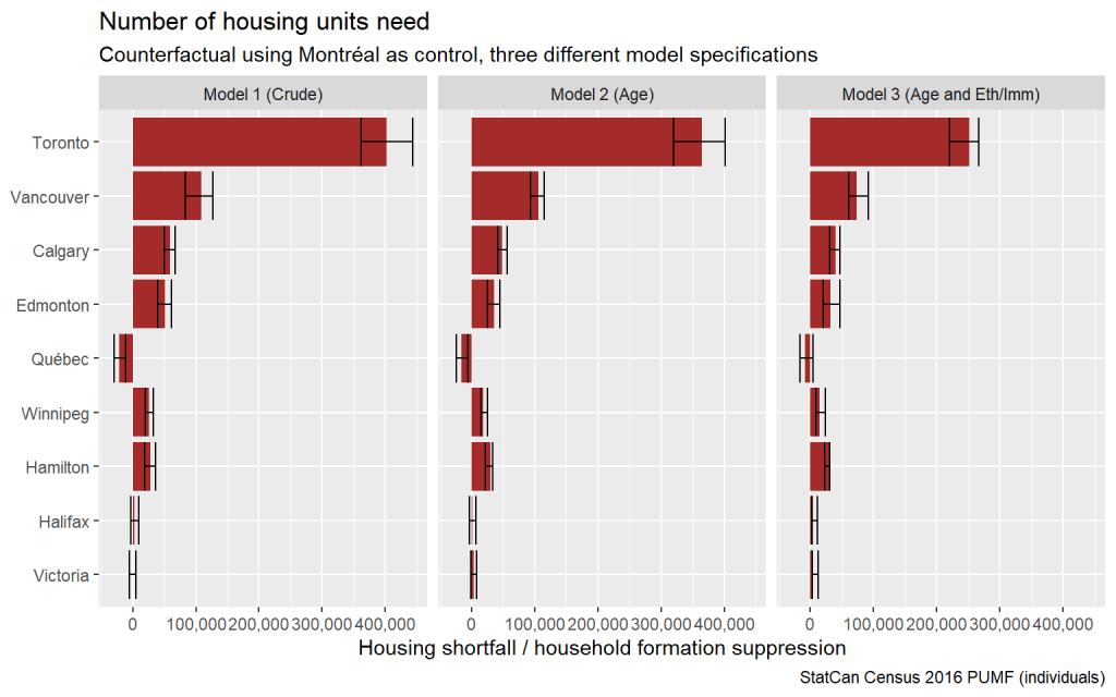
For Toronto, the Montréal Method estimates a housing shortfall of 250,000 to 400,000 dwellings, depending upon assumptions. For Vancouver, the shortfall range is narrower, from roughly 75,000 to 100,000 dwellings. We should stress again that this is only trying to estimate the housing shortage due to suppressed household formation, if we were to actually make up the dwelling shortfall this would almost certainly also alter migration patterns and interfere with these estimates.

At the national level we don’t have to worry about impacts of migration, if we are able to build the needed housing in all the right places. For all of Canada this housing shortfall comes out to around 890k units for our Model 2 and, if we are comfortable with our assumptions of adding culture into the model, 830k for our Model 3.

This includes the negative shortfall in Québec, which reminds us that maybe Montréal was already experiencing housing pressures in 2016 (which have intensified in the meantime) and perhaps isn’t the only counterfactual we should consider, leading to possible under-estimates. Indeed, if we look back to the age-based household maintainer rate timelines for Montréal we can observe a drop in household maintainer rates in the 20 to 39 year old age groups in the 2016 census supporting this. Still, if nothing else, Montréal provides us a conservative estimate of what less constrained household formation could look like.

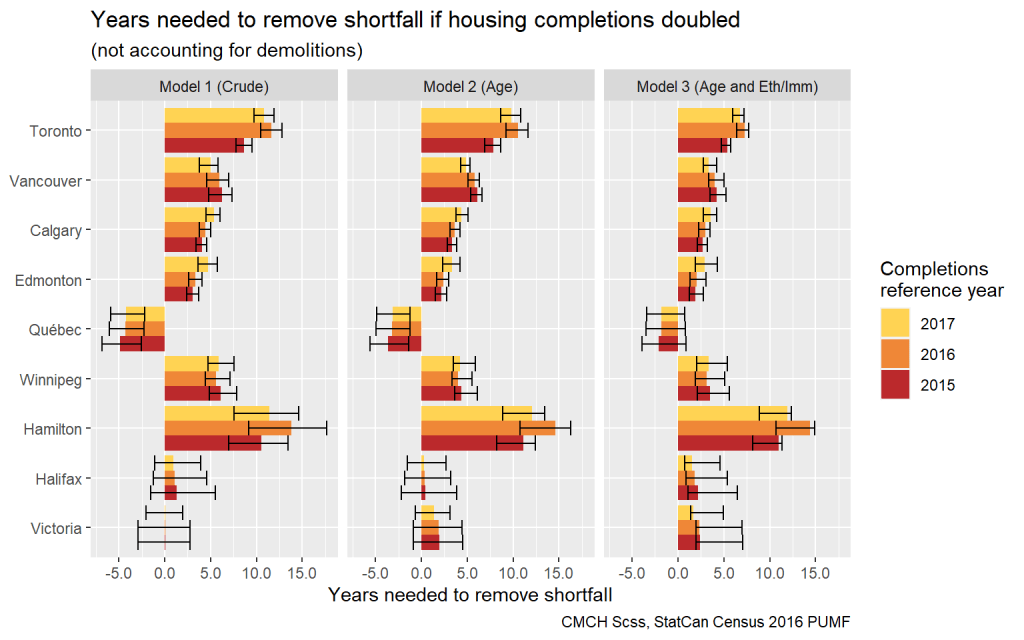
How could our estimated housing shortfall be fixed? To provide one last means of interpretation, we can compare our numbers above to the prevailing pace of housing completions. If we scaled up to the development industry to double the number of new dwellings completed circa 2016 – without accounting for demolitions – how long would it take to address the shortfall in each metro area?

How robust are these results?

This is a good start, but how realistic is our Model 3, and what might a more realistic Model 4 look like? And how would that effect the estimates?

We still have some concerns about Model 3. In particular, people are different both within and between any cultural groupings; hence assumptions about cultural groupings are tricky to get right. It’s difficult to adjust for possible differences in culture and living preferences between groups that also distribute themselves selectively across CMA. For example, people who move from places with large groups of co-ethnics to places with smaller groups may be distinct from those who stay in terms of their ideal living situations. This gets to a fundamental conundrum: the more realistic complexity we attempt to add to our model, the greater the risk we might make wrong assumptions about how that complexity actually works.

Possibly more realistic models

Given that we’ve laid out these risks, we can at least think through this a little more systematically and point at some other important factors we might want to consider if we want to add further complexity. We don’t have to worry about factors impacting just household maintainer rates as long as we think they don’t also impact, or are impacted by CMA in some way, and we will omit those. For example, we know that Gender impacts household maintainer rates, but we don’t believe CMA and Gender are strongly related, so for now we omit Gender from our model. We could model a set of important relationships as per below.

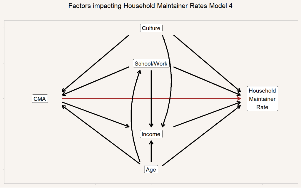
This model aims to capture the main effects impacting the relationship between CMA and Household Maintainer Rates, but still remains incomplete. It is still missing several factors that impact or confound the relationship between CMA and Household Maintainer Rates. For example, parental wealth likely interferes with household formation of young adults (e.g. the “gilded cage” effect) in ways that are not independent of CMA. The young adults in Vancouver and Toronto who don’t have help from parents in meeting their housing needs may choose at an increased rate to relocate to other CMAs and form households there. This kind of effect of people self-selecting into CMAs based on affordability issues would be captured broadly under CMA effects (and might increase noise).

Though there are factors missing, we don’t believe that they are necessarily correlated with the other factors, Age, Income, School/Work/Neither status, or Culture in our model. We’d certainly be interested in seeing how the factors we attempt to include might shift, e.g. the model hints at how adjusting for culture in our Model 3 may well soak up some income effects. Armed with a model like this we could use census data to estimate the effect of CMA on household maintainer rates. Two effects actually, the total effect, including the effect mediated through differences in the income distribution which we assume to be partially caused by CMA level variables, and the direct effect (in red) that is not mediated through CMA-induced differences in the income distribution.

But there’s a further problem. While this model probably does a better job at capturing the complexities, we can’t expect PUMF data to produce reasonable estimates. The PUMF’s 1:40 subsample is simply not deep enough for the complexity of the model. To stand a fighting chance to estimate this model we might need to use the full census data at the RDC. Having access to the census in the RDC would also allow to explore further linkages in the data and add features of parents into the model that might interact with CMA, for example type of dwelling the parents live in.

Upshot

We develop and elaborate the Montréal Method for estimating constrained household formation. Taken together, we interpret our results from applying the Method as evidence that housing shortage is likely constraining household formation quite a bit, especially in Toronto, but also Vancouver and elsewhere across Canada. Montréal makes for a decent and fun counterfactual, enabling us to estimate housing shortage. While it might have some cultural idiosyncrasies that limit its applicability as counterfactual, Montréal’s relatively stable and accessible (for Canada) vacancy rates; the fact that Halifax has similar overall household maintainer rates; and the fact that Montréal’s maintainer rates were quite similar to Toronto and Vancouver in the 1970s, all suggest the Montréal Method does its job ok.

We open up many more questions with our analysis so far. Returning to history, why did household maintainer rates change so much outside of Montréal, and how has this related to the housing market of other CMAs. While household maintainer rates remain useful, we may want to look at distinct lifecourse factors and situations to work this out in detail. For instance, we would like to spend more time observing the living arrangements of young adults at the ages 20 or 25 through 39 where the bulk of the household formation happens. Some transitions, e.g leaving home, tend to increase household formation, while others, e.g. coupling, reduce it. Connecting transitions to housing stock availability can offer deeper insight into the mechanisms by which household maintainer rates differ across regions, which can sometimes work in opposing ways. For example, Calgary has a lower rates of young adults living with their parents compared to Montreal, but a higher rate of young adults living as roommates. While these details are secondary to linking population to households, they offer important insights into the mechanisms behind household formation in different regions in Canada.

Another possibly fruitful angle of attack to identify the CMA effects in a more robust way in the face of our models getting entangled in complex revealed (constrained) preferences is to explicitly introduce prevailing levels of rent as a mediator between CMA and household maintainer rates and try to identify the effect mediated through rents.

We will explore some of this in a future blog post.

As usual, the code for this post is available on GitHub for anyone to replicate or adapt for their own purposes.

Appendix

PUMF data

Public use micro data (PUMF) is a (roughly) 1:40 representative subsample of individual level census responses, somewhat altered to preserve anonymity. This allows to generate flexible CMA level cross tabulations that we will need for more complex models, like the one including Culture. It is a good idea to do a cross-check to see how well the PUMF data lines up with the cross tabulation when just accounting for age to get a better understanding of the uncertainties and challenges when working with PUMF data.

To get a feel for how PUMF data compares to the full (25%) census data we compare the age-adjusted household maintainer rates by CMA estimated from the two different sources.

Generally they line up well. Here we pooled the 15-17 and 17-19 age groups in the PUMF to match the ones in the cross tabulation and added in the estimate based on standard weights in red. We do not that especially with the smaller CMAs we see wider confidence intervals from the PUMF estimates and some deviation.